
 |  |
|
|
Reading the Output of Print Commands in VisA model initially given as a Verilog description undergoes several transformations before Vis can run model checking on it. Vis provides several printing commands to inspect the various data structures. Oftentimes, the output of these commands is a bit obscure for the casual user, but with the "help" command, and the following example, one should be able to make sense of most of it.
Commands Related to the HierarchyLet us consider the following very simple description.
module parity (clk,i,o);
    input  clk;
    input  i;
    output o;
    reg    o;
    initial o = 0;
    always @ (posedge clk) o = o ^ i;
endmodule // fa
If we run this code through vl2mv, we get: # vl2mv parity.v # version: 0.2 # date: 19:54:06 05/20/01 () .model parity # I/O ports .outputs o .inputs i # o = 0 .names o$raw_n0 0 # non-blocking assignments for initial # o = o ^ i # o ^ i .names o i _n2 .def 0 0 1 1 1 0 1 .names _n2 o$raw_n1 - =_n2 # conflict arbitrators .names _n3 .def 0 1 .names _n3 o$raw_n1 _n4 .def 0 1 0 0 1 1 1 # non-blocking assignments # latches .r o$raw_n0 o 0 0 1 1 .latch _n4 o # quasi-continuous assignment .end When we read parity.mv into vis and type "print_hierarchy_stats" (or, using the aliases defined in master.visrc, "phs"), we get: vis release 1.4 (compiled 20-May-01 at 4:02 AM) vis> rlmv parity.mv vis> phs Model name = parity, Instance name = parity inputs = 1, outputs = 1, variables = 7, tables = 5, latches = 1, children = 0 Here the numbers of inputs, outputs, and latches should come as no surprise. Notice that clk is identified as the implicit
clock by vl2mv, and is not present in parity.mv.
The number of tables (5) is the number of ".names" in the .mv file.
The number of variables (7) reflects the fact that there are seven
variables in the .mv file; namely,
o, i, o$raw_n0, _n2, o$raw_n1, _n3, _n4.The number of children is 0 because no module is instantiated in parity. Other commands that are applicable at this stage are "print_latches" ("pl"), "print_io" ("pio"), and "print_models" ("pm"). vis> pl o vis> pio inputs: i outputs: o vis> pm Model name = parity inputs = 1, outputs = 1, variables = 7, tables = 5, latches = 1 subckts = 0 Commands Related to the NetworkWe now build the network for our design by calling "flatten_hierarchy" ("flt"), and then print stats about the result with "print_network_stats" ("pns").vis> flt vis> pns parity combinational=4 pi=1 po=1 latches=1 pseudo=0 const=1 edges=6 This summarizes what we get with "print_network" ("pn"): vis> pn Nodes of network parity: o$NS: mdd=-1, shadow; o$INIT: mdd=-1, combinational; constant initial-input comb-output _n2: mdd=-1, combinational; o: mdd=-1, latch; output comb-input comb-output _n4: mdd=-1, combinational; data-input comb-output i: mdd=-1, primary-input; comb-input o$raw_n1: mdd=-1, combinational; At this point, no MDDs/BDDs have been built for this network. Hence, we find mdd=-1 for all nodes of the network.
A few noteworthy things have happened in going from the hierarchy to
the network. First of all,
Second, some redundant nodes have been removed by constant
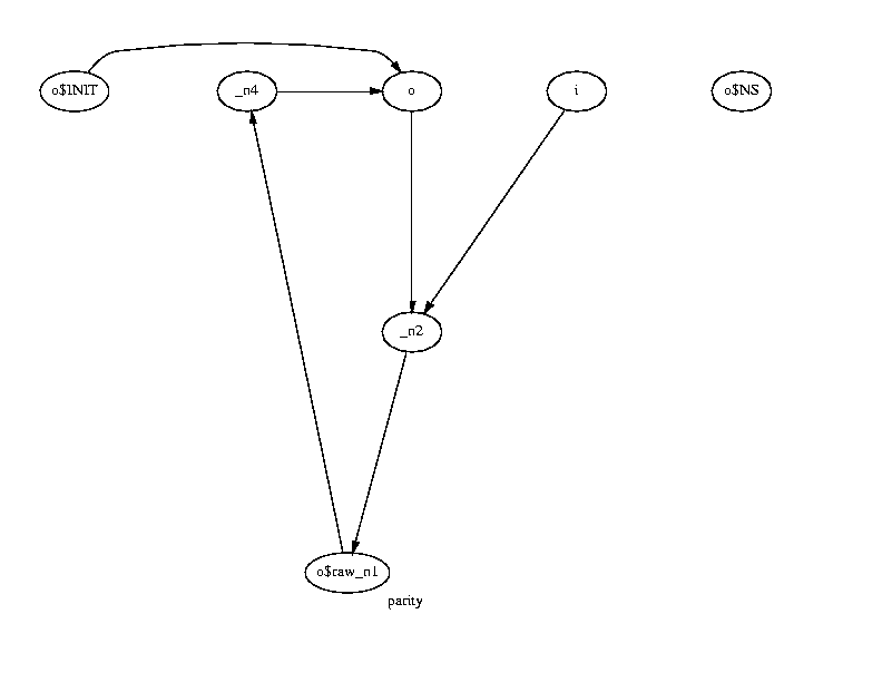
propagation, namely The number of edges is the total number of edges of the network graph or, as "help pns" explains, the total number of fanouts of each node. In our case the edges are: i -> _n2 _n2 -> o$raw_n1 o$raw_n1 -> _n4 _n4 -> o o$INIT -> o o -> _n2for a total of 6. This information can be obtained by typing "print_network_dot." (See below for a short discussion of dot.) 
We now run "static_order" to associate BDD variables to each comb-input. Let's see how this affects the output of "print_network." vis> so vis> pn Nodes of network parity: o$NS: mdd=2, shadow; o$INIT: mdd=-1, combinational; constant initial-input comb-output _n2: mdd=-1, combinational; o: mdd=1, latch; output comb-input comb-output _n4: mdd=-1, combinational; data-input comb-output i: mdd=0, primary-input; comb-input o$raw_n1: mdd=-1, combinational; We see that primary input, latch, and next state nodes have been assigned an MDD id. An MDD variable is a variable that can take a finite set of values. Each MDD variable corresponds to one or more BDD variables. In this case, all variables are two-valued; hence, each MDD variable corresponds to one (binary) BDD variable. The nodes that do not have MDD variables assigned to them still have mdd=-1.
Commands Related to the PartitionThe next step is "build_partition_mdds" ("part"). This command identifies a set of comb-inputs and comb-outputs (the partition) and builds MDDs for the comb-outputs in terms of the comb-inputs. (Some intermediate variables may be used as well for large networks, but we shall ignore this detail here.)MDDs are similar to BDDs. They differ in that their variables are multi-valued (e.g., a variable may take values BLUE, RED, and GREEN) instead of binary. MDDs are implemented as an abstraction layer on top of BDDs. So, building the MDDs boils down to building the BDDs for the network. We then use "print_partition_stats" to inquire about the result. vis> part vis> pps Method Frontier, 2 sinks, 3 sources, 4 total vertices, 4 mdd nodes We can get more information by passing the -n option.
vis> pps -n
Network nodes represented as vertices in the partition:
o
i
_n4
o$INIT
Method Frontier, 2 sinks, 3 sources, 4 total vertices, 4 mdd nodes
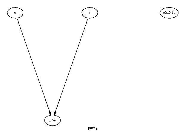
The partition gives the MDDs of _n4 in terms of o,
i. This is seen by examining the output of "print_partition"
("pp"). The partition, as explained by "help pp," is in the format of
the dot
graph layout program. Things like "rotate=90" are instructions to dot
on how to draw the graph. The details can be found in the
documentation of dot.
vis> pp
# vis release 1.4 (compiled 20-May-01 at 4:02 AM)
# partition name: parity
# generated: Sun May 20 14:57:57 2001
#
# Partition with 4 vertices and 2 edges
digraph "parity" {
  rotate=90;
  margin=0.5;
  label="parity";
  size="10,7.5";
  ratio="fill";
  node0 [label="o"];
  node1 [label="i"];
  node2 [label="_n4"];
  node3 [label="o$INIT"];
  node1 -> node2;
  node0 -> node2;
}
The result of running dot on the output of "pp" is the following drawing. Notice that "print_network_dot" and "print_partition" are practically restricted to small models. 
Node o$INIT is also part of the partition because the
initial state depends on it. Since it is a constant node, no variable
is associated to it. Node o$INIT is classified as both a
source and a sink of the graph, because it has neither incoming arcs
nor outgoing arcs.
As explained by "help pps," the number of MDD nodes is the total number for all the functions in the partition. Other Print CommandsVIS builds a transition relation from the partition MDDs to carry out model checking or reachability analysis. The transition relations for (forward) reachability analysis and (backward) model checking are in general (not in this case, though) slightly different, and VIS builds them on demand depending of the command to be executed. However, we can force VIS to build the forward transition relation by typing "print_image_info" ("pii"). For our circuit, it results in the following:vis> pii Printing Information about Image method: IWLS95 Threshold Value of Bdd Size For Creating Clusters = 5000 (Use "set image_cluster_size value" to set this to desired value) Verbosity = 0 (Use "set image_verbosity value" to set this to desired value) W1 = 6 W2 = 1 W3 = 1 W4 = 2 (Use "set image_W? value" to set these to desired values) Shared size of transition relation for forward image computation is 1 BDD nodes (1 components) It gives information on the image computation method in effect (IWLS95, rather than, for instance, hybrid), the values of some parameters used in heuristic algorithms (users almost never change them) and the total size of the transition relation. At this point, MDDs have disappeared, and everything is in terms of the underlying BDDs. In this case, there is only one node in the transition relation because from each of the two possible states, it is possible to transit to both states in one cycle. Also, since the transition relation is small, it is represented by a single BDD, in which the primary input variable has been existentially quantified. These two things together imply that the transition relation is the BDD that is always 1. The "print_fairness" ("pf") command shows what fairness constraints are in effect. vis> pf Fairness constraint: TRUE; In our case, we get TRUE because there are no fairness
constraints in effect. All (infinite) paths are fair because
TRUE holds infinitely often along every infinite path.
After "static_order" one can inspect statistics of the BDDs by typing "print_bdd_stats." The output of this command depends on the BDD package linked to Vis, and is described in that package's documentation. For CUDD, which is the default package, the documentation can be found here. A final class of print commands is used to display the values of the options for various Vis commands. (E.g., "print_ardc_options.") The documentation for each such command is given by help command. That is, to get information on the meaning of the options used in approximate reachability analysis, one types "help print_ardc_options." |