Frequency Response of the Running Average Filter

The frequency response of an LTI system is the DTFT of the impulse response,

H(ω) = ∑_{(m
= − ∞
to ∞)} h(m) e^{− jωm}.

The impulse response of an L-sample moving average is

h(n) = 1/L, for n = 0, 1, ..., L − 1

h(n) = 0, otherwise

Since the moving average filter is FIR, the frequency response reduces to the finite sum

H(ω) = (1/L) ∑_{(m
= 0 to L −
1)} e^{− jωm}..

We can use the very useful identity

to write the frequency response as

H(ω) = (1/L) (1 − e^{−
jω}^L)/(1 − e^{− jω}).

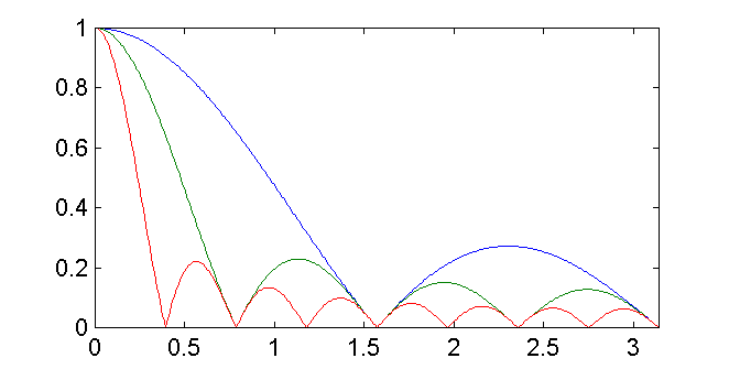
where we have let a = e^{−
jω}, N = 0, and M = L − 1. We may be interested in the magnitude of this function in order to determine which frequencies get through the filter unattenuated and which are attenuated. Below is a plot of the magnitude of this function for L = 4 (red), 8 (green), and 16 (blue). The horizontal axis ranges from zero to π radians per sample.

Notice that in all three cases, the frequency response has a lowpass characteristic. A constant component (zero frequency) in the input passes through the filter unattenuated. Certain higher frequencies, such as π /2, are completely eliminated by the filter. However, if the intent was to design a lowpass filter, then we have not done very well. Some of the higher frequencies are attenuated only by a factor of about 1/10 (for the 16 point moving average) or 1/3 (for the four point moving average). We can do much better than that.

The above plot was created by the following Matlab code:

omega = 0:pi/400:pi;
H4 = (1/4)*(1-exp(-i*omega*4))./(1-exp(-i*omega));
H8 = (1/8)*(1-exp(-i*omega*8))./(1-exp(-i*omega));
H16 = (1/16)*(1-exp(-i*omega*16))./(1-exp(-i*omega));
plot(omega,[abs(H4);abs(H8);abs(H16)])
axis([0, pi, 0, 1])

Week 12

Frequency Response of the Running Average Filter