5.2 An overview of SDF stars

The "open-palette" command in pigi ("O") will open a checkbox window that you can use to open the standard palettes in all of the installed domains. For the SDF domain, the star library is large enough that it has been divided into sub-palettes. The top-level palette is shown in figure 5-2

The "sources" palette contains signal generators of various types. The "sinks" palette contains various stars that display signals in different ways or write the value of signal samples to files. The "arithmetic" palette contains basic adders, subtracters, multipliers, and amplifiers, for all the standard scalar data types (floating point, complex, fixed-point, and integer). The "nonlinear" palette contains stars that compute transcendental functions, such as logarithm, cosine, sine, and exponential functions, as well as quantizer and table lookup stars. The "logic" palette contains stars that perform Boolean and comparison operations, such as and, or, and greater than. The "control" palette contains stars that manipulate the flow of tokens, such as commutators and distributors, downsamplers and upsamplers, and forks. The "conversion" palette contains stars that explicitly accomplish type conversion. The "matrix" palette contains matrix operators such as matrix addition and multiplication. More complex stars that use matrix operations internally can be found in other palettes, such as the singular value decomposition and Kalman filters in the "dsp" palette. The "matlab" palette contains stars that communicate with a Matlab process and thus have access to all of the functionality of Matlab. The "vis" palette contains stars that use the Sun UltraSparc Visual Instruction Set.The "dsp" palette contains various signal processing functions such as fixed and adaptive filters of various types. The "spectral" palette contains spectral estimation functions. The "communications" palette contains stars that are specific to digital communications functions, such as pulse shapers, speech coders, and QAM encoders. The "telecommunications" palette contains touchtone generators and decoders, channel models, and PCM coders. The "spatial array palette" contains models of sensors, Doppler effects, and beamformers. The "image" palette contains stars for image and video signal processing. The "neural" palette contains neural network stars. The "dfm" palette contains design flow management stars that use strings and files as datatypes. The "hof" palette contains the Higher Order Functions available in the SDF domain. The HOF stars in this palette are explained in detail in the HOF domain chapter. The "user" palette contains user contributed stars.

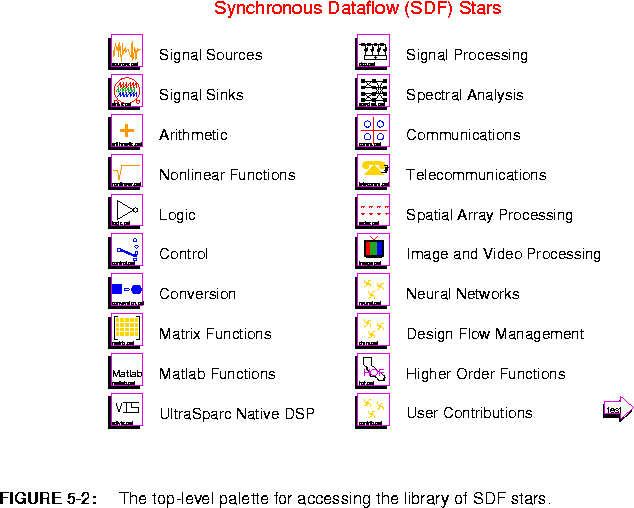
Each palette is summarized in more detail below. In the listing, whenever data types are not mentioned, double-precision floating point is used. Not all data types are represented in all stars. Type conversions, automatic or explicit, can be used to complete the collection.

The parameters of a star are shown in italics. More information about each star can be obtained using the on-line profile command (","), or the on-line man command ("M").

At the top of each palette, for convenience, are instances of the two delay icons, the bus icon, and the following star:

BlackHole Discard all inputs. This star is useful for discarding signals that are not useful.

The delay and bus icons are created on top of an arc to define its properties and are not stars.

5.2.1 Source stars

Source stars are stars with no inputs. They generate signals, and may represent external inputs to the system, constant data, or synthesized stimuli. In the dataflow model of computation, they are always enabled, and hence can be fired at any time. In the synchronous dataflow model, the frequency with which they are fired, relative to other stars in the system, is determined by the solution to the balance equations. The palette of source stars is shown in figure

5-3, and the stars are summarized below, in the order they appear in the palette.

Floating-point sources

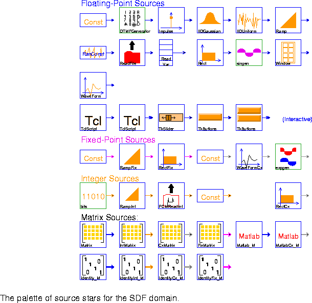
Const Output a constant signal with value given by the level parameter (default 0.0).
DTMFGenerator Create a dual-tone modulated-frequency signal, such as the tone generated by a touchtone telephone.
Impulse Generate a single impulse or an impulse train. Each impulse has an amplitude level (default 1.0). If period (default 0) is equal to 0, then only a single impulse is generated; otherwise, period specifies the period of the impulse train.
IIDGaussian Generate an identically independently distributed white Gaussian pseudo-random process with mean (default 0) and variance (default 1).
IIDUniform Generate an identically independently distributed uniformly distributed pseudo-random process. Output is uniformly distributed between lower (default 0) and upper (default 1).
Ramp Generate a ramp signal, starting at value (default 0.0) and incrementing by step size step (default 1.0) on each firing.
RanConst Generate an random number with a uniform(u), exponential(e), or normal(n) distribution, as determined by the distribution parameter. This star is new in Ptolemy 0.7.
ReadFile Read ASCII data from a file. The simulation can be halted on end-of-file, or the file contents can be periodically repeated, or the file contents can be padded with zeros.
ReadVar Output the value of a double-precision floating point variable from a shared memory. Use the writeVar star to write values into the shared memory. WARNING: This star may produce unpredictable results, since the results will depend on the precendences in the block diagram in which it appears as well as the scheduler used.
Rect Generate a rectangular pulse of height (default 1.0) and width (default 8). If period is greater than zero, then the pulse is repeated with the given period.
singen Generate a sine wave with frequency (relative to the given sample_rate) and phase given by phase_in_radians. This is implemented as a galaxy according to the formula
sin( 2 n frequency / sample_rate + phase_in_radians )
where n is the sample index. Therefore, frequency and sample_rate must have the same units, e.g. rad/sample, Hz, etc.
WaveForm Output a waveform as specified by the array state value (default "1 -1"). You can get periodic signals with any period, and can halt a simulation at the end of the given waveform. The following table summarizes the capabilities: haltAtEnd periodic period operation NO YES 0 The period is the length of the waveform NO YES N>0 The period is N NO NO anything Output the waveform once, then zeros YES anything anything Stop after outputting the waveform once The first line of the table gives the default settings. This star may be used to read a file by simply setting value to something of the form < filename, preferably specifying a complete path.
Window Generate standard window functions or periodic repetitions of standard window functions. The possible functions are: Rectangle, Bartlett, Hanning, Hamming, Blackman, Kaiser and SteepBlackman. One period of samples is produced at each firing.
TclScript (Two icons) Invoke a Tcl script that can optionally define a procedure that is invoked every time the star fires. That procedure can read the star's inputs and update the value of the outputs.
TkSlider Output a value determined by an interactive on-screen scale slider.
TkButtons This star outputs the value 0.0 on all outputs unless the corresponding button is pushed. When the button is pushed, the output takes the value given by the parameter value. If synchronous is YES, then outputs are produced only when some button is pushed. I.e., the star waits for a button to be pushed before its go method returns. If allow_simultaneous_events is YES, then the buttons pushed are registered only when the button labeled "PUSH TO PRODUCE OUTPUTS" is pushed. Note that if synchronous is NO, this star is nondeterminate.

haltAtEnd	periodic	period	operation
NO	YES	0	The period is the length of the waveform
NO	YES	N>0	The period is N
NO	NO	anything	Output the waveform once, then zeros
YES	anything	anything	Stop after outputting the waveform once

5-4 are those with no outputs. They display signals in various ways, or write them to files.

Batch Plotting Facilities

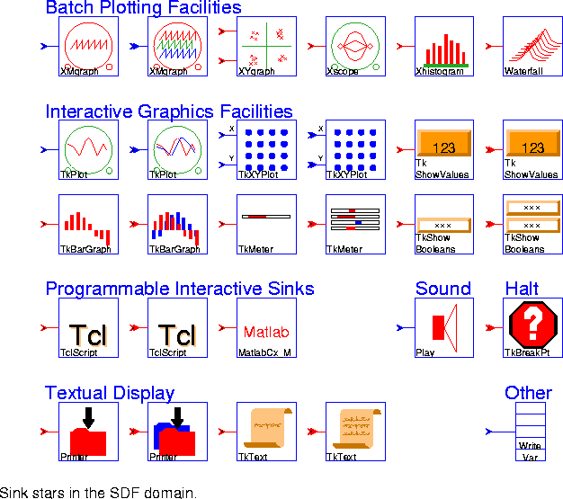
The first six stars in this palette are all based on the pxgraph program. This program has many options, summarized in "pxgraph - The Plotting Program" on page 20-1. The differences between stars often amount to little more than the choice of default options. Some, however, preprocess the signal in useful ways before passing it to the pxgraph program. The first allows only one input signal, the second allows any number (notice the double arrow on the input port).

XMgraph (two icons) Generate a generic multi-signal plot.
XYgraph Generate an X-Y plot with the pxgraph program. The X data is on "xInput" and the Y data is on "input".
Xscope Generate a multi-trace plot with the pxgraph program. Successive traces are overlaid on one another.
Xhistogram Generate a histogram with the pxgraph program. The parameter binWidth determines the bin width.
Waterfall Plot a series of traces in the style of a waterfall plot. This is a type of three-dimensional plot used to show the evolution of signals or spectra. Optionally, each plot can be made opaque, so that lines that would appear behind the plot are eliminated.

Interactive Graphics Facilities

These stars are multiple configurations of only six stars. These stars all use the Tk toolkit associated with the Tcl language to create interactive, animated displays on the screen.

TkPlot (two icons) Plot "Y" input(s) vs. time with dynamic updating. Two styles are currently supported: dot causes individual points to be plotted, whereas connect causes connected lines to be plotted. Drawing a box in the plot will reset the plot area to that outlined by the box. There are also buttons for zooming in and out, and for resizing the box to just fit the data in view.
TkXYPlot (two icons) Plot "Y" input(s) vs. "X" input(s) with dynamic updating. Two styles are currently supported: dot causes points to be plotted, whereas connect causes connected lines to be plotted. Drawing a box in the plot will reset the plot area to that outlined by the box. There are also buttons for zooming in and out, and for resizing the box to just fit the data in view.
TkShowValues (two icons) Display the values of the inputs in textual form. The print method of the input particles is used, so any data type can be handled, although the space allocated on the screen may need to be adjusted.
TkBarGraph (two icons) Dynamically display the value of any number of input signals in bar-chart form. The first 12 input signals will be assigned distinct colors. After that, the colors are repeated. The colors can be controlled using X resources.
TkMeter (two icons) Dynamically display the value of any number of input signals on a set of bar meters.
TkShowBooleans (two icons) Display input Booleans using color to highlight their value.

Programmable Interactive Sinks

TclScript (two icons) Invoke a Tcl script that can optionally define a procedure that is invoked every time the star fires. That procedure can read the star's inputs and update the value of the outputs.
MatlabCx_M Evaluate a Matlab function if inputs are given or evaluate a Matlab command if no inputs are given.

Sound

Play Play an input stream on the workstation speaker. This star works best on Suns, but can work on SGI Indigos and HP 700s and 800s. On HPs, you may need other publicly available software for this star to work. The gain parameter (default 1.0) multiplies the input stream before it is µ-law compressed and written. The inputs should be in the range of -32000.0 to 32000.0. The file is played at a fixed sampling rate of 8000 samples per second. When the wrapup method is called, a file of 8-bit µ-law samples is handed to a program named ptplay which plays the file. The ptplay program must be in your path. See "Sounds" on page 2-38 for more information.

Halt

TkBreakPt A conditional break point. Each time this star executes, it evaluates its conditional expression. If the expression evaluates to true, it causes the run to pause.

Textual Display

Printer (two icons) Print out one sample from each input port per line. The fileName parameter specifies the file to be written; the special names <stdout> and <cout> which specify the standard output stream, as well as <stderr> and <cerr> which specify the standard error stream, are also supported.
TkText (two icons) Display the values of the inputs in a separate window, keeping a specified number of past values in view. The print method of the input particles is used, so any data type can be handled.

Other

WriteVar Write the value of the input to a double-precision floating-point variable in shared memory. Use the ReadVar star to read values from the shared memory. WARNING: This star may produce unpredictable results, since the results will depend on the precedences in the block diagram in which it appears, as well as the scheduler (target) used.

5.2.3 Arithmetic stars

In principle, it should be possible to overload the basic arithmetic operators so that, for example, a single Add star could handle any data type. Our decision, however, was in favor of more explicit typing, in which there is an Add star for each particle type supported in the kernel. As before, when there is no data type suffix in the name of the star, the data type supported is double-precision floating point.

Many of the stars in this palette have more than one icon, as indicated in figure

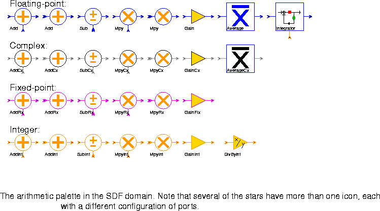
5-5. Each such icon has a different configuration of ports. This is done for visual clarity in schematics. A port with a double arrowhead can accept any number of input signals. Each four rows of the palette contains equivalent stars for floating-point, complex, fixed-point, and integer arithmetic, respectively. Listed by the roots of the names of the stars, they are:

Add (two icons) Output the sum of the inputs.
Sub Output the "pos" input minus all "neg" inputs.
Mpy (two icons) Output the product of the inputs.
Gain This is an amplifier; the output is the input multiplied by the gain (default 1.0).

The floating-point and complex-valued scalar data types also have the following star:

Average Average some number of input samples or blocks of input samples. Blocks of successive input samples are treated as vectors.

The floating-point type has one additional arithmetic star:

Integrator This is an integrator with leakage, limits, and reset. With the default parameters, input samples are simply accumulated, and the running sum is the output. To prevent any resetting in the middle of a run, connect a Const source with value 0 to the "reset" input. Otherwise, whenever a non-zero is received on this input, the accumulated sum is reset to the current input (i.e. no feedback).
Limits are controlled by the top and bottom parameters. If top £ bottom, no limiting is performed (this is the default). Otherwise, the output is kept between bottom and top. If saturate = YES, saturation is performed. If saturate = NO, wrap-around is performed (this is the default). Limiting is performed before output.
Leakage is controlled by the feedbackGain parameter (default 1.0). The output is the data input plus feedbackGain ¥ state, where state is the previous output.

The integer type has the following star:

DivByInt This is an amplifier. The integer "output" is the integer "input" divided by the integer divisor (default 1). Truncated integer division is used.

5.2.4 Nonlinear stars

The nonlinear palette (figure

5-6) in the SDF domain includes transcendental functions, quantizers, table lookup stars, and miscellaneous nonlinear functions.

Quantizers

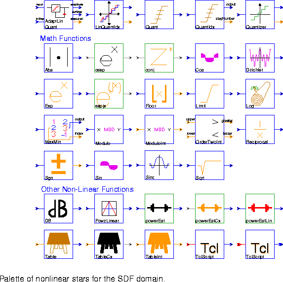
AdaptLinQuant Quantize the input to one of 2^bits possible output levels. The high and low output levels are anti-symmetrically arranged around zero and their magnitudes are determined by (2^bits-1)*"inStep"/2. The steps between levels are uniformly spaced at the step size given by the "inStep" input value. The linear quantizer can be made adaptive by feeding back past information such as quantization level, quantization value, and step size into the current step size.
LinQuantIdx Quantize the input to the number of levels given by the levels parameter. The quantization levels are uniformly spaced between low and high inclusive. Rounding down is performed, so that output level will equal high only if the input level equals or exceeds high. If the input is below low, then the quantized output will equal low. The quantized value is output to the "amplitude" port, while the index of the quantization level is output to the "stepNumber" port.
Quant Quantize the input value to one of N+1 possible output levels using N thresholds. For an input less than or equal to the n-th threshold, but larger than all previous thresholds, the output will be the n-th level. If the input is greater than all thresholds, the output is the N+1-th level. If level is specified, there must be one more level than thresholds; the default value for level is 0, 1, 2, ... N. This star is much slower than LinQuantIdx, so if possible, that one should be used instead.
QuantIdx Quantize the input value to one of N+1 possible output levels using N thresholds, and output both the quantized result and the quantization level. See the Quant star for more information.
Quantizer This star quantizes the input value to the nearest output value in the given codebook. The nearest value is found by a full search of the codebook, so the star will be significantly slower than either Quant or LinQuantIdx. The absolute value of the difference is used as a distance measure.

Math Functions

Abs Compute the absolute value of its input.
cexp Compute the complex exponential function of its complex input. See also expjx.
conj Compute the conjugate of its complex input.
Cos Compute the cosine of its input, assumed to be an angle in radians.
Dirichlet Compute the normalized Dirichlet kernel (also called the aliased sinc function):

The value of the normalized Dirichlet kernel at x = 0 is always 1, and the normalized Dirichlet kernel oscillates between -1 and +1. The normalized Dirichlet kernel is periodic in x with a period of either 2 when N is odd or 4 when N is even.
Exp Compute the real exponential function of its real input.
expjx Compute the complex exponential function of its real input. See also cexp.
Floor Output the greatest integer less than or equal to its input.
Log Output the natural logarithm of its input.
Limit The output of this star is the value of the input limited to the range between bottom and top inclusive.
MaxMin Finds maximum or minimum, value or magnitude, of a fixed number of data values on its input. If you want to use this star to operate over multiple data streams, then precede this star with a Commutator and set the parameter N accordingly.
Modulo The output is equal to the remainder after dividing the input by the modulo parameter.
ModuloInt The output is equal to the integer remainder after dividing the integer input by the integer modulo parameter.
OrderTwoInt Takes two inputs and outputs the greater and lesser of the two integers.
Reciprocal Output the reciprocal of its input, with an optional magnitude limit. If the magnitude limit is greater than zero, and the input value is zero, then the output will equal the magnitude limit.
Sgn Compute the signum of its input. The output is ±1. Note that 0.0 maps into 1.
Sin Computes the sine of its input, assumed to be an angle in radians.
Sinc Computes the sinc of its input given in radians. The sinc function is defined as sin(x)/x, with value 1.0 when x = 0.
Sqrt Computes the square root of its input.

Other Nonlinear Functions

DB Convert input to a decibels (dB) scale. Zero and negative values are assigned the value min (default -100). The inputIsPower parameter should be set to YES if the input signal is a power measurement (vs. an amplitude measurement).
PcwzLinear This star implements a piecewise linear mapping from the list of (x,y) pairs, which specify the breakpoints in the function. The sequence of x values must be increasing. The function implemented by the star can be represented by drawing straight lines between the (x,y) pairs, in sequence. The default mapping is the `tent' map, in which inputs between -1.0 and 0.0 are linearly mapped into the range -1.0 to 1.0. Inputs between 0.0 and 1.0 are mapped into the same range, but with the opposite slope, 1.0 to -1.0. If the input is outside the range specified in the "x" values of the breakpoints, then the appropriate extreme value will be used for the output. Thus, for the default map, if the input is -2.0, the output will be -1.0. If the input is +2.0, the output will again be -1.0.
powerEst Estimate the power in decibels (dB) by filtering the square of the input using a first-order filter with the time constant given as a number of sample periods.
powerEstCx Like powerEst, but for complex inputs.
powerEstLin Same as powerEst, but the output is on a linear scale instead of decibels (dB).
Table This star implements a real-valued lookup table indexed by an integer-valued input. The input must lie between 0 and N-1, inclusive, where N is the size of the table. The values parameter specifies the table. Its first element is indexed by a zero-valued input. An error occurs if the input value is out-of-bounds.
TableCx Table lookup for complex values.
TableInt Table lookup for integer values.
TclScript (two icons) Invoke a Tcl script that can optionally define a procedure that is invoked every time the star fires. That procedure can read the star's inputs and update the value of the outputs.

5.2.5 Logic stars

The logic palette shown in figure

5-7 is made up of only three stars. Each star has multiple icons representing a variety of configurations.

Test (four icons) Compare two inputs. The test condition can be any of {EQ NE GT GE} or {== != > >=}, resulting in equals, not equals, greater than, or greater than or equals. The four icons represent these possibilities.
If crossingsOnly is TRUE, then the output is non-zero only when the outcome of the test changes from TRUE to FALSE or FALSE to TRUE. In this case, the first output is always TRUE.
Multiple (one icon) Output a 1 if top input is a multiple of bottom input.
Logic (19 icons) This star applies a logical operation to any number of inputs. The inputs are integers interpreted as Booleans, where zero is a FALSE and nonzero is a TRUE. The logical operations supported are {NOT, AND, NAND, OR, NOR, XOR, XNOR}, with any number of inputs.

5.2.6 Control stars

Control stars (figure

5-8) manipulate the flow of tokens. All of these stars are polymorphic; they operate on any data type. From left to right, top to bottom, they are:

Single-Rate Operations

Fork (five icons) Copy input particles to each output. Note that a fork is automatically inserted in a schematic when a single output is sent to more than one input. However, when a delay is needed on one of the connections, then an explicit fork star must be used.
Reverse On each execution, read a block of N samples (default 64) and write them out backwards.
Transpose Transpose a rasterized matrix (one that is read as a sequence of particles, row by row, and written in the same form). The number of particles produced and consumed equals the product of samplesInaRow and numberOfRows.
TkBreakPt A conditional break point. Each time this star executes, it evaluates its conditional expression. If the expression evaluates to true, it causes the run to pause.
Trainer Pass the value of the train input to the output for the first trainLength samples, then pass the decision input to the output. This star is designed for use with adaptive equalizers that require a training sequence at start-up, but it can be used whenever one sequence is used during a start-up phase, and another sequence after that.

Multirate Operations

Commutator (four icons) Synchronously combine N input streams (where N is the number of inputs) into one output stream. The star consumes B input particles from each input (where B is the blockSize), and produces N ¥ B particles on the output. The first B particles on the output come from the first input, the next B particles from the next input, etc.
DownSample Decimate by a given factor (default 2). The phase tells which sample of the last factor samples to output. If phase = 0 (by default), the most recent sample is the output, while if phase = factor -1 the oldest sample is the output. Note that phase has the opposite sense of the phase parameter in the UpSample star, but the same sense as the phase parameter in the FIR star.
Distributor (four icons) Synchronously split one input stream into N output streams, where N is the number of outputs. The star consumes N ¥ B input particles, where B is the blockSize parameter, and sends the first B particles to the first output, the next B particles to the next output, etc.
Repeat Repeat each input sample a specified number of times.
UpSample Upsample by a given factor (default 2), giving inserted samples the value fill (default 0.0). The phase parameter (default 0) tells where to put the sample in an output block. A phase of 0 says to output the input sample first, followed by the inserted samples. The maximum phase is equal to factor - 1. Although the fill parameter is a floating-point number, if the input is of some other type, such as complex, then the fill particle will be obtained by casting fill to the appropriate type.

Other Operations

Chop On each execution, this star reads a block of nread particles and writes them to the output with the given offset. The number of particles written is given by nwrite. The output block contains all or part of the input block, depending on offset and nwrite. The offset specifies where in the output block the first (oldest) particle in the input block will lie. If offset is positive, then the first offset output particles will be either particles consumed on previous firings (if use_past_inputs parameter is YES), or zero (otherwise). If offset is negative, then the first offset input particles will be discarded.
ChopVarOffset This star has the same functionality as the Chop star except the offset parameter is determined at run time by a control input.
DeMux (two icons) Demultiplex one input onto any number of output streams. The star consumes B particles from the input, where B is the blockSize. These B particles are copied to exactly one output, determined by the "control" input. The other outputs get a zero of the appropriate type.
Integers from 0 through N - 1 are accepted at the "control" input, where N is the number of outputs. If "control" is outside this range, all outputs get zeros.
Mux (two icons) Multiplex any number of inputs onto one output stream. B particles are consumed on each input, where B is the blockSize. But only one of these blocks of particles is copied to the output. The one copied is determined by the "control" input. Integers from 0 through N - 1 are accepted at the "control" input, where N is the number of inputs. If "control" is outside this range, an error is signaled.

5.2.7 Conversion stars

The palette in figure

5-9 shows a collection of stars for format conversions of various types. The first two rows contain stars with functions that are fundamentally different from the automatic type conversion performed by Ptolemy. From left to right, top to bottom, they are:

Complex data type formats

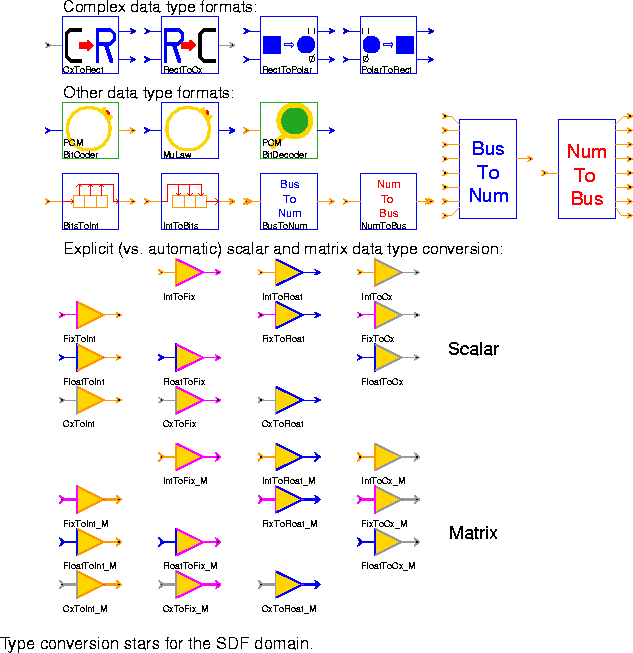
CxToRect Convert a complex input to real and imaginary parts.
RectToCx Convert real and imaginary inputs to a complex output.
RectToPolar Convert real and imaginary inputs into magnitude and phase form. The phase output is in the range - to .
PolarToRect Convert magnitude and phase to rectangular form.

Other data type formats

PCMBitCoder Encode voice samples for a 64 kbps bit stream using CCITT Recommendation G.711. The input is one 8 kHz sample of voice data and the output is the eight-bit codeword (the low-order 8 bits of an integer) representing the quantized samples.
MuLaw This star encodes its input into an 8 bit representation using the nonlinear companding µ-law. It is similar to PCMBitCoder, but it does the conversion in a single star, rather than a galaxy.
PCMBitDecoder Decode 8-bit PCM codewords that were encoded using PCMBitCoder.
BitsToInt The integer input sequence is interpreted as a bit stream in which any non-zero value is a "1" bit. This star consumes nBits successive bits from the input, packs them into an integer, and outputs the resulting integer. The first received bit becomes the most significant bit of the output. If nBits is larger than the integer wordsize, then the first bits received will be lost. If nBits is smaller than the wordsize minus one, then the output integer will always be non-negative.
IntToBits Read the least significant nBits bits from an integer input, and output the bits as integers serially on the output, most significant bit first.
BusToNum (two icons) This star accepts a number of input bit streams, where this number should not exceed the word size of an integer. Each bit stream has integer particles with values 0, 3, or anything else. These are interpreted as binary 0, tri-state, or 1, respectively. When the star fires, it reads one input bit from each input. If any of the input bits is tri-stated, the output will be the previous output (or the initial value of the previous parameter if the firing is the first one). Otherwise, the bits are assembled into an integer word, assuming two's complement encoding, and sign extended. The resulting signed integer is sent to the output. This star is particularly useful for interfacing to digital logic simulation domains.
NumToBus (two icons) This star accepts an integer and outputs the low-order bits that make up the integer on a number of outputs, one bit per output. The number of outputs should not exceed the word size of an integer. This star is particularly useful for interfacing to digital logic simulation domains.

Automatic type conversion, as implemented in Ptolemy 0.7, has limitations. If a given output port has more than one destination, then all destinations must have the same type input. This is true even if an explicit fork star is used. Explicit type conversions are needed to get around this limitation. For this reason, the palette in figure 5-9 also contains a set of type conversions that behave exactly the same way the automatic type conversions behave.

IntToFix Convert an integer input to a fixed-point output.
IntToFloat Convert an integer input to a floating-point output.
IntToCx Convert an integer input to a complex output.
FixToInt Convert a fixed-point input to an integer output.
FixToFloat Convert a fixed-point input to a floating-point output.
FixToCx Convert a fixed-point input to a complex output.
FloatToInt Convert a floating-point input to an integer output.
FloatToFix Convert a floating-point input to a fixed-point output.
FloatToCx Convert a floating-point input to a complex output.
CxToInt Convert a complex input to an integer output.
CxToFix Convert a complex input to a fixed-point output.
CxToFloat Convert a complex input to a floating-point output.

Matrix Conversion Stars

The following type conversions construct a new matrix of the destination type by converting each element of the old matrix as it is copied to the new one. For FixMatrix types, the precision is specified as a parameter of the conversion star. The actual conversions are implemented using the cast conversion in the underlying class, except for the conversions to the FixMatrix type which are more complex because they involve possible changes in precision and require a rounding option. The stars provided are:

IntToFix_M Convert an integer input matrix to a fixed-point output matrix.
IntToFloat_M Convert an integer input matrix to a floating-point output matrix.
IntToCx_M Convert an integer input matrix to a complex output matrix.
FixToInt_M Convert a fixed-point input matrix to an integer output matrix.
FixToFloat_M Convert a fixed-point input matrix to a floating-point output matrix.
FixToCx_M Convert a fixed-point input matrix to a complex output matrix.
FloatToInt_M Convert a floating-point input matrix to an integer output matrix.
FloatToFix_M Convert a floating-point input matrix to a fixed-point output matrix.
FloatToCx_M Convert a floating-point input matrix to a complex output matrix.
CxToInt_M Convert a complex input matrix to an integer output matrix.
CxToFix_M Convert a complex input matrix to a fixed-point output matrix.
CxToFloat_M Convert a complex input matrix to a floating-point output matrix.

5.2.8 Matrix stars

The stars in the matrix palette (figure

5-10) operate on particles that represent matrices with floating-point, fixed-point, complex, or integer entries. Most of the work is done in the underlying matrix classes, FloatMatrix, ComplexMatrix, FixMatrix, and IntMatrix. These classes are treated as ordinary particles. In Pigi, matrix types are indicated with thick terminal stems, where the color of the terminal stem corresponds to the data type of the matrix elements.

The Matrix conversion stars are in the conversion palette, see "Matrix Conversion Stars" on page 5-22 for more information.

Matrix-Vector Conversion

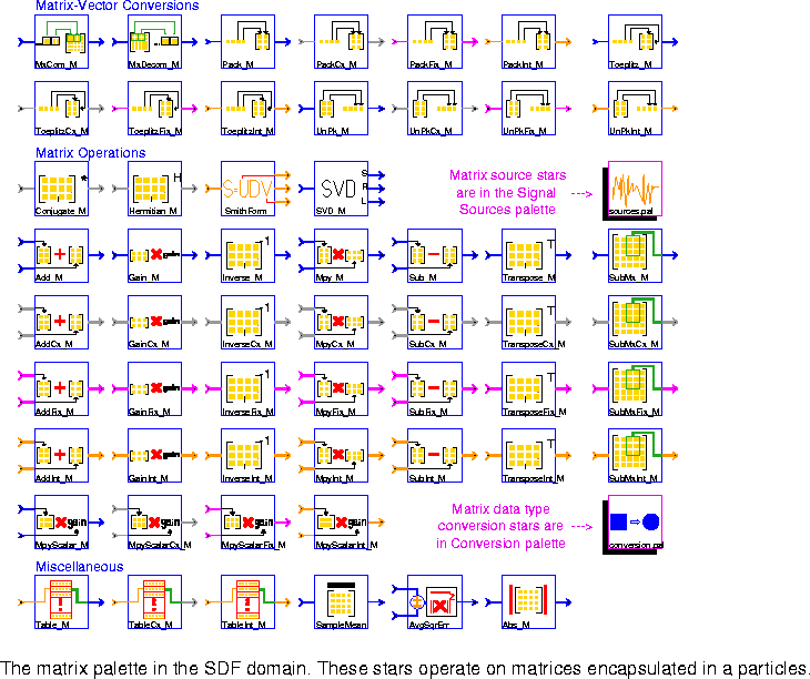
MxCom_M Accept input matrices and create a matrix output. Each input matrix represents a decomposed submatrix of output matrix in row by row. Note that for one output image, we will need a total (numRows / numRowsSubMx) ¥ (numCols / numColsSubMx) input matrices.
MxDecom_M Decompose a portion of input matrix into a sequence of submatrices. The desired portion of input matrix is specified by the parameters startRow, startCol, numRows, and numCols. Then output each submatrix with dimension numRowsSubMx ¥ numColsSubMx in row by row. Note that for one input matrix, there will be a total of (numRows / numRowsSubMx) ¥ (numCols / numColsSubMx) output matrices.

The following conversions perform more interesting functions. They also come in four versions, one for each data type, and again we only list the floating-point version.

Pack_M (4 icons) Produce a matrix with floating-point entries constructed from floating-point input particles. The inputs are put in the matrix in rasterized order, e.g. for a M ¥ N matrix, the first row is filled from left to right using the first N input particles.
Toeplitz_M (4 icons ) Generate a floating-point data matrix X, with dimensions (numRows,numCols), from a stream of numRows + numCols - 1 input particles organized as shown below:

Here numRows = N - M + 1 and numCols = M. This Toeplitz matrix is the form of the matrix that is required by the SVD_M star, among others.
UnPk_M (4 icons) Read a floating-point matrix and output its elements, row by row, as a stream of floating-point particles.

Matrix operations

The following blocks are functions defined only for the ComplexMatrix data type.

Conjugate_M Conjugate a matrix.
Hermitian_M Perform a Hermitian transpose (conjugate transpose) on the input matrix.

The following blocks also appear in the signal processing palette.

SmithForm Decompose an integer matrix S into one of its Smith forms S = UDV, where U, D, and V are simpler integer matrices. The Smith form decomposition for integer matrices is analogous to singular value decomposition for floating-point matrices.
SVD_M Compute the singular-value decomposition of a Toeplitz data matrix A by decomposing A into A = UWV', where U and V are orthogonal matrices, and V' represents the transpose of V. W is a diagonal matrix composed of the singular values of A, and the columns of U and V are the left and right singular vectors of A.

See "Matrix Sources" on page 5-8 for the Matrix source stars.

The following are usual matrix operations. They are arranged row by row, with one row for each data type (floating point, complex, fixed point, and integer). We list below only the floating point data type, from left to right.

Add_M Add two floating-point matrices.
Gain_M Multiply a floating-point matrix by a static scalar gain value.
Inverse_M Invert a square floating-point matrix.
Mpy_M Multiply two floating-point matrices A and B to produce matrix C. Matrix A has dimensions (numRows,X). Matrix B has dimensions (X,numCols). Matrix C has dimensions (numRows,numCols). The user need only specify numRows and numCols. An error will be generated if the number of columns in A does not match the number of rows in B.
Sub_M Subtract floating-point matrix B from A.
Transpose_M Transpose a floating-point matrix read as a single particle.
SubMx_M Find a submatrix of the input matrix.
MpyScalar_M Multiply a floating-point matrix by a scalar gain value given in parameter.

Miscellaneous

Table_M (3 stars for floating-point, complex and integer) This star implements a lookup table indexed by an integer-valued input. The output is a matrix. The input must lie between 0 and N - 1, inclusive, where N is the number of matrices in the table. The floatTable parameter specifies the entries of matrices in the table. Note that the entries of each matrix in the table should be given in row major ordering. The first matrix in the table is indexed by a zero-valued input. An error occurs if the input value is out of bounds.
SampleMean Find the average amplitude of the components of the input matrix.
AvgSqrErr Find the average squared error between two input sequences of matrices.
Abs_M Return the absolute value of each entry of the floating-point matrix.

5.2.9 Matlab stars

The Matlab stars provide an interface between Ptolemy and Matlab, a numeric computation and visualization environment from The Math Works, Inc. Each Matlab star can contain a single Matlab function, command, statement, or several statements. Ptolemy handles the conversion of inputs into Matlab format and the results from Matlab into Ptolemy format. For the Matlab stars to work, Matlab version 4.1 or later must be installed. Matlab is not distributed with Ptolemy ¹. If a Matlab star is run and Matlab is not installed, then Ptolemy will report an error. All Matlab stars send their commands to the same Matlab process.

Xavier Warzee of Thomson-CSF provided a method of running Matlab on a remote machine and obtaining the results from within Ptolemy. If a simulation needs to start Matlab, then the PTMATLAB_REMOTE_HOST environment variable is checked. If this variable is set, then its value is assumed to be the name of the remote machine to run Matlab on. The remote Matlab process is started up with the Unix rsh command. Once the remote process is running, if the MATLAB_SCRIPT_DIR environment variable is set, then its value is passed to the remote Matlab process as part of the command

path(path.'MATLAB_SCRIPT_DIR')

where MATLAB_SCRIPT_DIR is the value of that variable on the local machine.

Internally, Matlab distinguishes between real matrices and complex matrices. As a consequence, in Figure 5-11

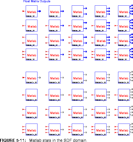
there are two types of Matlab stars: one outputs floating-point matrices and one outputs complex-valued matrices. These stars can take any number of inputs provided that the inputs have the same data type (floating point or complex). The two types of Matlab stars are:

Matlab_M Evaluate a Matlab expression and output the result as floating-point matrices.
MatlabCx_M Evaluate a Matlab expression and output the result as complex-valued matrices.

The implementation of Matlab stars is built on Matlab's engine interface. The interface is managed by a base star, SDFMatlab. The base star does not have any inputs or outputs. It provides methods for starting and killing a Matlab process, evaluating Matlab commands, managing Matlab figures, changing directories in Matlab, and passing Ptolemy matrices in and out of Matlab. Currently, the base star does support real- and complex-valued matrices, but not Matlab's other two matrix data types, sparse and string matrices.

Figures generated by a Matlab star are managed according to the value of the star's DeleteOldFigures parameter. If TRUE or YES, then the Matlab star will close any plots, graphics, etc., that it has generated when the Matlab star is destroyed (e.g., when the run panel in the graphical interface is closed). Otherwise, the figures remain until Ptolemy exits. For standalone programs generated by compile-SDF, it is better to set this parameter to NO so that the plots will not disappear when then standalone programs finishes.

There are several ways in which Matlab commands can be specified in the Matlab stars. The Matlab stars Matlab_M and MatlabCx_M have a parameter MatlabFunction. If only a Matlab function name is given for this parameter, then the function is applied to the inputs in the order they are numbered and the output(s) of the function is (are) sent to the star's outputs. For example, specifying eig means to perform the eigendecomposition of the input. The function will be called to produce one or two outputs, according to how many output ports there are. If there is a mismatch in the number of inputs and/or outputs between the Ptolemy star and the Matlab function, Ptolemy will report the error generated by Matlab.

The user may also specify how the inputs are to be passed to a Matlab function or how the outputs are taken from the Matlab function. For example, consider a two-input, two-output Matlab star to perform a generalized eigendecomposition. The command

[output#2, output#1] = eig( input#2, input#1 )

says to perform the generalized eigendecomposition on the two input matrices, place the generalized eigenvectors on output#2, and the eigenvalues (as a diagonal matrix) on output#1. Before this command is sent to Matlab, the pound characters `#' are replaced with underscore `_' characters because the pound character is illegal in a Matlab variable name.

The Matlab stars also allow a sequence of commands to be evaluated. Continuing with the previous example, we can plot the eigenvalues on a graph after taking the generalized eigendecomposition:

[output#2, output#1] = eig( input#2, input#1 );
plot( output#1 )

When entering such a collection of commands in Ptolemy, both commands would appear on the same line without a newline after the semicolon. In this way, very complicated Matlab commands can be built up. We can make the plot of eigenvalues always appear in the same plot without interfering with other plots generated by other Matlab stars:

[output#2, output#1] = eig( input#2, input#1 );
if ( exist(`myEigFig') == 0 ) myEigFig = figure; end;
figure(myEigFig);
plot( output#1);

For more information about using Matlab stars, please refer to the Matlab demonstrations.

5.2.10 UltraSparc Native DSP

The Visual Instruction Set (VIS) demos only run on Sun Ultrasparc workstations with the Sun unbundled CC compiler and a Ptolemy tree that has been compiled with the PTARCH variable set to sol2.5.cfront. The VIS demos will not work the Gnu compilers. You must have the Sun Visual Instruction Set Development kit installed, see http://www.sun.com/sparc/vis/vsdkfaq.html.

The palette shown in figure 5-12 has icons for the library of Sun UltraSparc Visual Instruction Set (VIS) stars

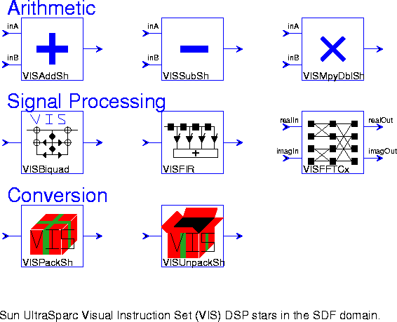
VISAddSh Add the shorts in a 16 bit partitioned float to the corresponding shorts in a 16 bit partitioned float. The result is four signed shorts that is returned as a single floating point number. There is no saturation arithmetic so that overflow results in wraparound.
VISSubSh Subtract the shorts in a 16 bit partitioned float to the corresponding shorts in a 16 bit partitioned float.The result is four signed shorts that is returned as a single floating point number. There is no saturation arithmetic so that overflow results in wraparound.
VISMpyDblSh Multiplies the shorts in a 16 bit partitioned float to the corresponding shorts in a 16 bit partitioned float. The result is four signed shorts that is returned as a single floating point number. Each multiplication results in a 32 bit result, which is then rounded to 16 bits.
VISBiquad An IIR Biquad filter.
VISFIR A finite impulse response (FIR) filter.
VISFFTCx A single complex sequence FFT using radix 2.
VISPackSh Pack four floating point numbers into a single floating point number.
VISUnPackSh Unpack a single floating point number into four floating point numbers.

5.2.11 Signal processing stars

The palette shown in figure

5-13 has icons for the library of signal processing functions. Simple time-domain filtering operations come first.

Filters

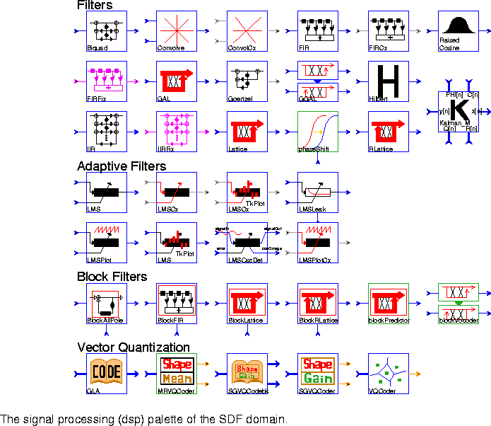
Biquad A two-pole, two-zero Infinite Impulse Response filter (a biquad). The default is a Butterworth filter with a cutoff at 0.1 times the sample frequency. The transfer function is
.
Convolve Convolve two causal finite sequences of floating point numbers. The truncationDepth parameter specifies the number of terms used in the convolution sum. Set truncationDepth larger than the number of output samples of interest.
ConvolveCx Convolve two causal finite sequences of complex numbers. The truncationDepth parameter specifies the number of terms used in the convolution sum. Set truncationDepth larger than the number of output samples of interest.
FIR A Finite Impulse Response (FIR) filter. Coefficients are specified by the taps parameter. The default coefficients give an 8th order, linear-phase, lowpass filter. To read coefficients from a file, replace the default coefficients with < fileName, preferably specifying a complete path. Rational sampling rate changes, implemented by polyphase multirate filters, is also supported.
FIRCx A complex FIR filter. Coefficients are specified by the taps parameter. The default coefficients give an 8th order, linear phase, lowpass filter. To read coefficients from a file, use the syntax: < fileName, preferably specifying a complete path. Real and imaginary parts should be paired with parentheses, e.g. (1.0, 0.0). Polyphase multirate filtering is also supported.
RaisedCosine An FIR filter with a magnitude frequency response that is shaped like the standard raised cosine or square-root raised cosine used in digital communications. By default, the star upsamples by a factor of 16, so 16 outputs will be produced for each input unless the interpolation parameter is changed.
FIRFix An FIR filter with fixed-point capabilities. The fixed-point coefficients are specified by the taps parameter. The default coefficients give an 8th order, linear phase lowpass filter. To read coefficients from a file, replace the default coefficients with < fileName, preferably specifying a complete path. Polyphase multirate filtering is also supported.
Kalman_M Output the state vector estimates of a Kalman filter using a one- step prediction algorithm.
GAL A Gradient Adaptive Lattice filter.
Goertzel Second-order recursive computation of the kth coefficient of an N-point DFT using Goertzel's algorithm.
GGAL Ganged Gradient Adaptive Lattice filters.
Hilbert Output the (approximate) Hilbert transform of the input signal. This star approximates the Hilbert transform by using an FIR filter, and is derived from the FIR star.
IIR An Infinite Impulse Response (IIR) filter implemented in direct form II. The transfer function is of the form
,
where N() and D() are polynomials. The parameter gain specifies G, and the floating-point arrays numerator and denominator specify N() and D(), respectively. Both arrays start with the constant terms of the polynomial and decrease in powers of z (increase in powers of 1/z). Note that the constant term of D is not omitted, as is common in other programs that assume it is always normalized to unity.
IIRFix This is a fixed-point version of the IIR star. The coefficient precision, input precision, accumulation precision, and output precision can all be separately specified.
Lattice An FIR lattice filter. The default reflection coefficients form the optimal predictor for a particular 4th-order AR random process. To read other reflection coefficients from a file, replace the default coefficients with < fileName, preferably specifying a complete path.
phaseShift This galaxy applies a phase shift to a signal according to the "shift" input. If the "shift" input value is time varying, then its slope determines the instantaneous frequency shift.
RLattice A recursive (IIR) lattice filter. The default coefficients implement the synthesis filter for a particular 4th-order AR random process. To read reflection coefficients from a file, replace the default coefficients with < fileName, preferably specifying a complete path.

Adaptive Filters

LMS An adaptive filter using the Least-Mean Square (LMS) adaptation algorithm. The initial coefficients are given by the taps parameter. The default initial coefficients give an 8th order, linear phase lowpass filter. To read default coefficients from a file, replace the default coefficients with < fileName, preferably specifying a complete path. This star, which is derived from FIR, supports decimation, but not interpolation.
LMSCx Complex version of the LMS star.
LMSCxTkPlot This star is just like the LMSCx star, but with an animated Tk display of the taps, plus associated controls.
LMSLeak An LMS adaptive filter in which the step size is input (to the "step" input) every iteration. In addition, the mu parameter specifies a leakage factor in the updates of the filter coefficients.
LMSPlot This star is just like the LMS star, except that, in addition to the functions of LMS, it makes a plot of the tap coefficients. It can produce two types of plots: a plot of the final tap values or a plot that traces the time evolution of each tap value. The time evolution is obtained if the value of the parameter trace is YES.
LMSTkPlot This star is just like the LMS star, but with an animated Tk display of the taps, plus associated controls.
LMSOscDet This filter tries to lock onto the strongest sinusoidal component in the input signal, and outputs the current estimate of the cosine of the frequency of the strongest component and the error signal. It is a three-tap LMS filter whose first and third coefficients are fixed at one. The second coefficient is adapted. It is a normalized version of the Direct Adaptive Frequency Estimation Technique.
LMSPlotCx Complex version of LMSPlot. Separate plots are generated for the magnitude and phase of the filter coefficients.

Block Filters

The next group of stars perform "block filtering", which means that on each firing, they read a set of input particles all at once, process them, and produce a set of output particles. The number of particles in a set is specified by the blockSize parameter.

BlockAllPole This star implements an all pole filter with the denominator coefficients of the transfer function externally supplied. For each set of coefficients, a block of input samples is processed, all in one firing. The transfer function is

where the coefficients of are externally supplied.
BlockFIR This star implements an FIR filter with coefficients that are periodically updated from the outside. For each set of coefficients, a block of input samples is processed, all in one firing.
BlockLattice A block forward lattice filter. It is identical to the Lattice star except that the reflection coefficients are updated each time the star fires by reading the "coefs" input. The order parameter indicates how many coefficient should be read. The blockSize parameter specifies how many data samples should be processed for each set of coefficients.
BlockRLattice A block recursive (IIR) lattice filter. It is identical to the RLattice star, except that the reflection coefficients are updated each time the star fires by reading the "coefs" input. The order and blockSize parameters have the same interpretation as in the BlockLattice star.
blockPredictor A block predictor galaxy used in speech processing.
blockVocoder A block vocoder galaxy.

Vector Quantization

Quantization is the heart of converting analog signals to digital signals. Traditional techniques are based on scalar coding which quantizes symbols, such as pixels in images, one by one. On the other hand, vector quantization can perform better by operating the quantization on groups of symbols instead of individual symbols.

GLA Use the Generalized Lloyd Algorithm (GLA) to yield a codebook from input training vectors. Note that each input matrix will be viewed as a row vector in row by row. Each row of output matrix represents a codeword of the codebook.
MRVQCoder Mean removed vector quantization coder.
SGVQCodebk Jointly optimized codebook design for shape-gain vector quantization. Note that each input matrix will be viewed as a row vector in row by row. Each row of first output matrix represents a codeword of the shape codebook. Each element of the second output matrix represents a codeword of the gain codebook.
SGVQCoder Shape-gain vector quantization encoder. Note that each input matrix will be viewed as a row vector in row by row.
VQCoder Full search vector quantization encoder. It consists in finding the index of the nearest neighbor in the given codebook corresponding to the input matrix. Note that each input matrix will first be viewed as a row vector in row by row, in order to find the nearest neighbor codeword in the codebook.

5.2.12 Spectral analysis

The group of stars shown in figure

5-14 are concerned with various signal analysis algorithms.

autocorrelation Estimate a power spectrum using the autocorrelation method, a method that uses the Levinson-Durbin algorithm to compute linear predictor coefficients, and then uses these coefficients to construct an approximate maximum entropy power spectrum estimate.
blockFFT An overlap and add implementation of the FFT.
burg Estimate a power spectrum using Burg's method, a method that computes linear predictor coefficients, and then uses them to construct a maximum entropy power spectrum estimate.
Burg This star uses Burg's algorithm to estimate the linear predictor coefficients of an input random process. These coefficients are produced both in autoregressive form (on the "lp" output) and in lattice filter form (on the "refl" output). The "errPower" output is the power of the prediction error as a function of the predictor order. This star is used in the burg galaxy.
DB Convert input to a decibel (dB) scale. Zero and negative values are assigned the value min (default -100). The inputIsPower parameter should be set to YES if the input signal is a power measurement (vs. an amplitude measurement).
DTFT Compute the discrete-time Fourier transform (DTFT) at frequency points specified on the "omega" input.
FFTCx Compute the discrete-time Fourier transform of a complex input using the fast Fourier transform (FFT) algorithm. The parameter order (default 8) is the log base 2 of the transform size. The parameter size (default 256) is the number of samples read (<= 2^order). The parameter direction (default 1) is 1 for the forward, -1 for the inverse FFT.
GoertzelPower Second-order recursive computation of the power of the kth coefficient of an N-point DFT using Goertzel's algorithm. This form is used in touch-tone decoding.
LevDur This star uses the Levinson-Durbin algorithm to compute the linear predictor coefficients of a random process, given its autocorrelation function as an input. These coefficients are produced both in autoregressive form (on the "lp" output) and in lattice filter form (on the "refl" output). The "errPower" output is the power of the prediction error as a function of the predictor order.
MUSIC_M This star is used to estimate the frequencies of some specified number of sinusoids in a signal. The output is the eigenspectrum of a signal, such that the locations of the peaks of the eigenspectrum correspond to the frequencies of the sinusoids in the signal. The input is the right singular vectors in the form generated by the SVD_M star. The MUSIC algorithm (multiple signal characterization) is used.
periodogram Estimate a power spectrum using the periodogram method. This consists in computing the magnitude squared of the DFT of a set of observations of the signal. The FFT algorithm is used.
SmithForm Decompose an integer matrix S into one of its Smith forms S = UDV, where U, D, and V are simpler integer matrices. The Smith form decomposition for integer matrices is analogous to singular value decomposition for floating-point matrices.
SVD_M Compute the singular-value decomposition of a Toeplitz data matrix A by decomposing A into A = UWV', where U and V are orthogonal matrices, and V' represents the transpose of V. W is a diagonal matrix composed of the singular values of A, and the columns of U and V are the left and right singular vectors of A.
Unwrap Unwraps a phase plot, removing discontinuities of magnitude 2. This star assumes that the phase never changes by more than in one sample period. It also assumes that the input is in the range [-,].
Window Generate standard window functions or periodic repetitions of standard window functions. The possible functions are Rectangle, Bartlett, Hanning, Hamming, Blackman, SteepBlackman, and Kaiser. One period of samples is produced on each firing. This star is also found in the signal sources palette.

Miscellaneous signal processing blocks

Autocor Estimate an autocorrelation function by averaging input samples. Both biased and unbiased estimates are supported.
PattMatch This star accepts a template and a search window. The template is slid over the window one sample at a time, and cross correlations are calculated at each step. The cross-correlations are output on the "values" output. The "index" output is the value of the time-shift which gives the largest cross correlation. This index refers to a position on the search window beginning with 0 corresponding to the earliest arrived sample of the search window that is part of the best match with the template.

5.2.13 Communication stars

The limited set of communication stars that have been developed are shown in

figure 5-15, and summarized below. Many of these are galaxies, and should be viewed as examples of systems that a user can create.

Sources and pulse shapers

bits Produce "0" with probability probOfZero, else produce "1".
cosine.pal Produce a cosine waveform whose energy is normalized with respect to Amplitude. It is used in simulations for binary frequency shift keying (BFSK) demonstrations. This galaxy differs from the cosine star which computes the cosine of the input signal (see "Nonlinear stars" on page 5-13 for more information on the cosine star).
Hilbert Output the approximate Hilbert transform of the input signal. This star approximates the Hilbert transform by using an FIR filter, and is derived from the FIR star. The Hilbert star is also in the signal processing palette, which is discussed on page 5-30.
RaisedCosine An FIR filter with a magnitude frequency response shaped like the standard raised cosine or square-root raised cosine used in digital communication. By default, the star upsamples by a factor of 16, so 16 outputs will be produced for each input unless the interpolation parameter is changed.
RaisedCosineCx This galaxy uses the RaisedCosine star to implement an FIR filter for complex inputs with a raised cosine or square-root raised cosine transfer function.

Transmitter functions

NR2Zero Binary to Nonreturn-to-Zero Signaling Converter
QAM4 Encode an input bit stream into a 4-QAM (or 4-PSK) complex symbol sequence.
QAM16 Encode an input bit stream into a 16-QAM complex symbol sequence.
Scrambler Scramble the input bit sequence using a feedback shift register. The taps of the feedback shift register are given by the polynomial parameter, which should be a positive integer. The n-th bit of this integer indicates whether the n-th tap of the delay line is fed back. The low-order bit is called the 0-th bit, and should always be set. The next low-order bit indicates whether the output of the first delay should be fed back, etc. The default polynomial is an octal number defining the V.22bis scrambler.
Spread Frame synchronized direct-sequence spreader.
xmit2fsk Binary frequency shift keying (BFSK) transmitter.
xmit2pam Simple 2-level pulse amplitude modulation (PAM) transmitter.
xmit4pam Simple 4-level pulse amplitude modulation (PAM) transmitter.
xmit2psk Binary 2-level phase shift keying (BPSK) Modulator.
xmitspread Direct-sequence spreader (i.e., spread-spectrum transmitter).

Receiver functions

DeScrambler Descramble the input bit sequence using a feedback shift register. The taps of the feedback shift register are given by the polynomial parameter. This is a self-synchronizing descrambler that will exactly reverse the operation of the Scrambler star if the polynomials are the same. The low-order bit of the polynomial should always be set.
DeSpreader Frame synchronized direct-sequence despreader.
hilbertSplit This galaxy implements a phase splitter, in which the real-valued input signal is converted to an (approximate) analytic signal. The signal is filtered by the Hilbert block to generate the imaginary part of the output, while the real part is obtained by creating a matching delay.
qam4Slicer This galaxy implements a slicer (decision device) for a 4-QAM (or equivalently, 4-PSK) signal. The output decision is a complex number with +1 or -1 for each of the real or imaginary parts.
qam16Slicer This galaxy implements a slicer (decision device) for a 16-QAM complex signal. The output decision is a complex number with +1, -1, +3, or -3 for each of the real or imaginary parts.
qam16Decode A 16-QAM decoder similar to the CCITT V22.bis standard. The quadrant is differentially de-encoded.
phaseShift Shifts the phase of the input signal on the in input by the shift value on the shift input. The phase shifting is implemented by filtering the input signal with a complex FIR filter to convert it into an analytic signal and the complex result is modulated by a complex exponential. If the shift value is time varying, then its slope determines the instantaneous frequency shift.
rec2fsk Binary frequency shift keying (BFSK) Receiver.
rec2pam Simple 2-level pulse amplitude modulation (PAM) receiver.
rec4pam Simple 4-level pulse amplitude modulation (PAM) receiver.
rec2psk Binary pulse shift keying (BPSK) Demodulator.
recspread Direct sequence receiver.

Channel models

AWGNchannel Model an additive Gaussian white noise channel with optional linear distortion.
basebandEquivChannel Baseband equivalent channel.
freqPhase Impose frequency offset and/or phase jitter on a signal in order to model channels, such as telephone channels, that suffer these impairments.
noiseChannel A simple channel model with additive Gaussian white noise.
nonLinearDistortionGenerate second and third harmonic distortion by squaring and cubing the signal, and adding the results in controlled proportion to the original signal.
telephoneChannel 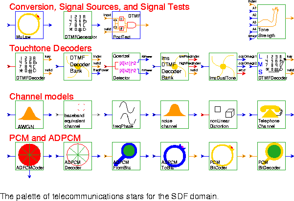Simulate impairments commonly found on a telephone channel, including additive Gaussian noise, linear and nonlinear distortion, frequency offset, and phase jitter.

5.2.14 Telecommunications

The telecommunications stars are in figure 5-16

Conversion, Signal Sources, and Signal Tests

MuLaw Transform the input using a logarithmic mapping if the compress parameter is true. In telephony, applying the µ-law to eight-bit sampled data is called companding, and it is used to quantize the dynamic range of speech more accurately. The transformation is defined in terms of the non-negative integer parameter mu: output = log (1 + mu | input | ) / log( 1 + mu )
DTMFGenerator Generate a dual-tone modulated-frequency (DTMF) signal by adding a low frequency and a high frequency sinusoid together. DTMF tones only consist of first harmonics. The default parameters generate a "1" on a touchtone telephone.
PostTest Return whether or not a valid dual-tone modulated-frequency has been correctly detected based on the last three detection results.
ToneStrength Decision circuit for dual-tone modulated-frequency (DTMF) decoding. It returns true if Amax is greater than or equal to Ai for i = 1, 2, 3, 4 such that i does not equal index.

Touchtone Decoders

DTMFDecoder Dual-tone modulated-frequency (DTMF) decoder based on post-processing of a bank of Goertzel discrete Fourier transform filters. This galaxy decodes touch tones generated by a telephone.
DTMFDecoderBank Implement one of the banks for detecting dual-tone frequency-modulated (DTMF) touch tones. Touch tones are generated by adding a low frequency and a high frequency sinusoid together. The galaxy is used to detect either the low or high frequency component, depending on the parameter settings. This algorithm examines the magnitude of the expected frequency components and their second harmonics. DTMF tones do not have second harmonics, so if they are present, then the input is likely speech and not touch tones. The valid output is true if the input is probably a touch tone. The default parameters are used to detect the low frequency tones.
GoertzelDetector Detect the energy of the first and second harmonic using a pair of Goertzel filters.
lmsDTMFDecoderBank Dual-tone modulated frequency detection based on the post-processing of the output of two LMS algorithms in cascade. These two algorithms are used to detect the two strongest frequencies present in the signal.
lmsDualTone Detect the location of the two strongest harmonic components in the input signal for every input sample using the normalize direct frequency estimation technique, which is based on the LMS algorithm. This galaxy is used in touchtone detection.
lmsDTMFDecoder Least-mean squares dual-tone modulated-frequency decoder. Dual-tone modulated frequency detection based on the post-processing of the output of two LMS algorithms in cascade. These two algorithms are used to detect the two strongest frequencies present in the signal.

Channel Models

For more complete descriptions, see the channel models for the communications stars given on page 5-36.

AWGN Simulate a channel with additive Gaussian noise.
basebandEquivChannel Baseband equivalent channel.
freqPhase Impose frequency offset and/or phase jitter on a signal in order to model channels, such as telephone channels, that suffer these impairments.
noiseChannel A simple channel model with additive Gaussian white noise.
nonLinearDistortion Generate second and third harmonic distortion by squaring and cubing the signal, and adding the results in controlled proportion to the original signal.
TelephoneChannel Telephone channel simulator with Gaussian noise and nonlinear distortion.

PCM and ADPCM

ADPCMCoder Implement adaptive differential pulse code modulation using an LMS star. Both the quantized and unquantized prediction-error signals are available as outputs.
ADPCMDecoder Decode the quantized prediction error signal produced by the ADPCMCoder galaxy.
ADPCMFromBits Convert a bit stream encoded with the ADPCMToBits galaxy back to floating-point values. The 4 low-order bits of the input integer are changed to 1 of 16 floating-point values scaled by range.
ADPCMToBits Convert the quantized prediction error of the ADPCMCoder galaxy into a bit stream. The quantized prediction error has 16 possible levels, so this galaxy produces 4 bits in each output sample.
PCMBitCoder 64kps PCM encoder (CCITT Recommendation G.711).
PCMBitDecoder 64kps PCM encoder (CCITT Recommendation G.711).

5.2.15 Spatial Array Processing

The spatial array processing stars given here support a single demonstration named RadarChainProcessing developed by Karim Khiar from Thomson CSF. The radar simulation, though five-dimensional, is implemented using SDF, which is a one-dimensional dataflow model. The stars on this palette are shown in figure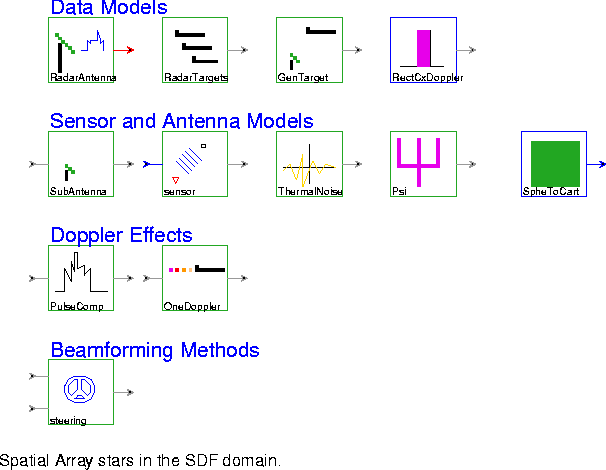

5-17.

Data Models

RadarAntenna Generate a specified number of Doppler filter outputs. This galaxy consists of a cascade of a network of antennas, a bank of matched filters, a bank of windows, and a Doppler filter. The bank of matched filters convolves the antenna outputs with a filter matched to a complex pulse train.
RadarTargets Model the observed data as the addition of the receive signal plus sensor noise. The received signal consists of a summation of the emissions of all of the targets.
GenTarget Model the reception of signals by one sensor. A complex pulse train is delayed and then multiplied by a complex exponential.
RectCx Generate a rectangular pulse of width "width" (default 240). If "period" is greater than zero, then the pulse is repeated with the given period.

Sensor and Antenna Models

SubAntenna Models a subantenna. It multiplies the input by a complex exponential.
sensor Compute the excitation of a plane wave arriving at a sensor at the given position with the arrival angle specified as an input. Position (0,0) is assumed to receive phase zero for any angle of arrival.
ThermalNoise Generate thermal noise as a complex noise process whose real and imaginary components are identically independently distributed Gaussian random processes.
Psi Model subantenna excitation.
SpheToCart Compute the inner product of two vectors, one given by a magnitude and two angles in spherical components, the other given by three cartesian components.

Doppler Effects

PulseComp This galaxy generates any number of targets and performs pulse compression. It uses the original chirp to perform the pulse compression. This output represents the output of the radar processing along the range bin axis. The y-axis represents the target magnitude on a linear, logarithmic scale.
OneDoppler Generate one Doppler output. This galaxy performs an antenna to pulse multiprojection transformation followed by a decimator.

Beamforming Methods

steering Multiply a sensor signal by a window sample and apply a steering correction.

5.2.16 Image processing stars

The image processing stars contained in the palette in figure 5-18

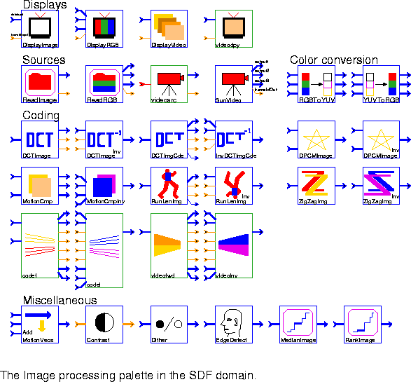
were originally written by Paul Haskell. For the Ptolemy 0.6 release, the image processing infrastructure was rewritten by Bilung Lee to use matrices as the underlying image representation. Since the stars are using the Matrix particle now, some old stars that are just doing simple matrix operation, such as SumImage, are removed, and we can use the matrix stars instead, such as Add_M.

Displaying images

DisplayImage Accept a black-and-white input grayimage represented by a float matrix and generate output in PGM (portable graymap) format. Send the output to a user-specified command (by default, xv is used). The user can set the root filename of the displayed image (which will probably be printed in the image display window title bar) and can choose whether or not the image file is saved or deleted. The image frame number is appended to the root filename in order to form the complete filename of the displayed image.
DisplayRGB This is similar to DisplayImage, but accepts three color images (Red, Green, and Blue) from three input float matrix and generates a PPM (portable pixmap) format color image file. The image file is displayed using a user-specified command (by default, xv is used).
DisplayVideo Accept a stream of black-and-white images from input float matrix, save the images to files, and display the resulting files as a moving video sequence. This star requires that programs from the Utah Raster Toolkit (URT) be in your path. Although this toolkit is not included with Ptolemy, it is available for free. See this star's long description (with the "look-inside" or "manual" commands in the Ptolemy menu) for information on how to get the toolkit.
The user can set the root filename of the displayed images (which probably will be printed in the display window title bar) with the ImageName parameter. If no filename is set, a default will be chosen.
The Save parameter can be set to YES or NO to choose whether the created image files should be saved or deleted. Each image's frame number is appended to the root filename in order to form the image's complete filename.
The ByFields parameter can be set to either YES or NO to choose whether the input images should be treated as interlaced fields that make up a frame or as entire frames. If the inputs are fields, then the first field should contain frame lines 1, 3, 5, etc. and the second field should contain lines 0, 2, 4, 6, etc.
videodpy Display an image sequence in an X window. This is simply the SDFDisplayVideo star encapsulated in a galaxy so that it can be easily used in other domains.

Reading images

ReadImage Read a sequence of PGM-format images from different files and send them out in a float matrix.
If present, the character # in the fileName parameter is replaced with the frame number to be read next. For example, if the frameId parameter is set to 2 and if the fileName parameter is dir.#/pic# then the file that is read and output is dir.2/pic2.
ReadRGB Read a PPM-format image from a file and send it out in three different images- a Red, Green, and Blue image. Each image is represented in a float matrix. The same mechanism for reading successive frames as in ReadImage is supported.
videosrc Read in an image from a specified file. This is simply the SDFReadImage star encapsulated in a galaxy so that it can be easily used in other domains.
SunVideo Reads frames from the SunVideo card and outputs them as 3 matrices: one for Y,U and V components. This star is new in Ptolemy 0.7, and does not yet have any demos.

Color conversions

RGBToYUV Read three float matrices that describe a color image in RGB format and output three float matrices that describe an image in YUV format. No downsampling is done on the U and V signals.
YUVToRGB Read three float matrices that describe a color image in YUV format and output three float matrices that describe an image in RGB format.

Image and video coding

DCTImage Take a float matrix input particle, compute the discrete cosine transform (DCT), and output a float matrix.
DCTImageInv Take a float matrix input, compute the inverse discrete cosine transform (DCT), and output a float matrix.
DCTImgCde Take a float matrix which represents a DCT image, insert "start of block" markers, run-length encode it, and output the modified image.
For the run-length encoding, all values with absolute value less than the Thresh parameter are set to 0.0, to help improve compression. Runlengths are coded with a "start of run" symbol and then an (integer) run-length.
The HiPri parameter determines the number of DCT coefficients per block are sent to "hiport", the high-priority output. The remainder of the coefficients are sent to "loport", the low-priority output.
InvDCTImgCde Read two coded float matrices (one high priority and one low-priority), invert the run-length encoding, and output the resulting float matrix. Protection is built in to avoid crashing even if some of the coded input data is affected by loss.
DPCMImage Implement differential pulse code modulation of an image. If the "past" input is not a float matrix or has size 0, pass the "input" directly to the "output". Otherwise, subtract the "past" from the "input" (with leakage factor alpha) and send the result to "output".
DPCMImageInv This star inverts differential pulse code modulation of an image. If the "past" input is not a float matrix or has size 0, pass the "diff" directly to the "output". Otherwise, add the "past" to the "diff" (with leakage factor alpha) and send the result to "output".
MotionCmp If the "past" input is not a float matrix (e.g. dummyMessage), copy the "input" image unchanged to the "diffOut" output and send a null field (zero size matrix) of motion vectors to "mvHorzOut" and "mvVertOut" outputs. This should usually happen only on the first firing of the star.
For all other inputs, perform motion compensation and write the difference frames and motion vector frames to the corresponding outputs.
This star can be used as a base class to implement slightly different motion compensation algorithms. For example, synchronization techniques can be added or reduced-search motion compensation can be performed.
MotionCmpInv For NULL inputs (zero size matrices) on "mvHorzIn" and/or "mvVertIn", copy the "diffIn" input unchanged to "output" and discard the "pastIn" input. (A NULL input usually indicates the first frame of a sequence.)
For non-NULL "mvHorzIn" and "mvVertIn" inputs, perform inverse motion compensation and write the result to "output".
RunLenImg Accept a float matrix and run-length encode it. All values closer than Thresh to meanVal are set to meanVal to help improve compression. Run lengths are coded with a start symbol of meanVal and then a run-length between 1 and 255. Runs longer than 255 must be coded in separate pieces.
RunLenImgInv Accept a float matrix and inverse run-length encode it.
ZigZagImage Zig-zag scan a float matrix and output the result. This is useful before quantization.
ZigZagImageInv Inverse zig-zag scan a float matrix.
codef This galaxy encodes a sequence of images using motion compensation, a discrete-cosine transform, quantization, and run-length encoding. The outputs are split into high priority and low priority, where corruption of the low priority data will impact the image less.
codei This galaxy inverts the encoding of the codef block, and outputs a reconstructed image sequence.
videofwd This galaxy is obsolete and will probably disappear in the next release.
videoinv This galaxy is obsolete and will probably disappear in the next release.

Miscellaneous image blocks

AddMotionVecs Over each block in the input image, superimpose an arrow indicating the size and direction of the corresponding motion vector.
Contrast Enhance the contrast in the input image by histogram modification. Input image should be in an integer matrix. The possible contrast type are Uniform (default) and Hyperbolic.
Dither Do digital halftoning (dither) of input image for monochrome printing. Input image should be in a float matrix. The possible dither methods are Err-Diffusion (default), Clustered, Dispersed, and Own. If you specify Own, then you can use your own dither mask.
EdgeDetect Detect edges in the input image. Input image should be in a float matrix. The possible detectors are Sobel (default), Roberts, Prewitt, and Frei-Chen.
MedianImage Accept an input grayimage represented by a float matrix, median-filter the image, and send the result to the output. Filter widths of 1, 3, 5 work well. Any length longer than 5 will take a long time to run.
Median filtering is useful for removing impulse-type noise from images. It also smooths out textures, so it is a useful pre-processing step before edge detection. It removes inter-field flicker quite well when displaying single frames from a moving sequence.
RankImage Accept an input grayimage represented by a float matrix, rank filter the image, and send the result to the output. A common example of a rank filter is the median filter, e.g. MedianImage, which is derived from this star. Pixels at the image boundaries are copied and not rank filtered.

5.2.17 Neural Networks

The neural network stars demonstrate logic functions using classical artificial neurons and McCulloch-Pitts neuron. These stars were written by Biao Lu (The University of Texas at Austin), Brian L. Evans (The University of Texas at Austin), and are present in Ptolemy 0.7 and later.The neural network stars are shown in figure

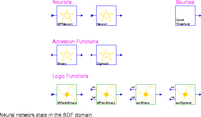
MPNeuron This is a McCulloch-Pitts neuron. The activation of this neuron is binary. That is, at any time step, the neuron either fires, or does not fire.
Neuron This neuron will output the sum of the weighted inputs, as a floating value.
ConstThreshold Output a constant signal with value given by the "level" parameter (default 0.0)
Binary Binary threshold of the input.
Sigmoid Compute the Sigmoid function, defined as 1/(1 + exp(-r*input)), where r is the learning rate.
MPandBinary The fact that the McCulloch-Pitts neuron is a digital device makes this neuron well-suited to the representation of a two-valued logic, such as AND, OR, and NAND.
MPxorBinary This example shows that a network of McCulloch-Pitts neurons has the power of the finite state automaton known as a Turing machine.
xorBinary XOR function can be implemented by a three-layer neural network which consists of an input layer, a hidden layer and an output layer. A binary activation function is used.
xorSigmoid XOR function can be implemented by a three-layer neural network which consists of an input layer, a hidden layer and an output layer. A sigmoid activation function is used.

Most of the stars that interface to Tcl appear in palettes that reflect their function. For instance, all the stars beginning with Tk in the "sinks" palette are actually Tcl stars derived from TclScript. This is the most generic Tcl star, with no useful function on its own. It must have a Tcl script associated with it to make it useful. There is a chapter of the Programmer's Manual of the The Almagest devoted to how to write such scripts. The complete palette of Tcl stars, which includes many stars that also appear in other palettes, is shown in figure

5-20. These stars, although derived from TclScript, assume the presence of the Tk graphics toolkit. For descriptions of the display and "sink" stars, see Sections 5.2.1 and 5.2.2, respectively.

¹ Contact The Math Works, Inc., Cochituate Place, 24 Prime Park Way, Natick, Mass. 01760-1500, USA, Phone: (508) 653-1415. Their Web site is http://www.mathworks.com/.